Using Neural Networks and Combinatorial Cross-Validation for Stock Strategies
Using Neural Networks and Combinatorial Cross-Validation for Stock Strategies
This post draws from Chapter 7 of the remarkable book Advances in Financial Machine Learning by Marcos Lopez de Prado.
Cross-validation plays a critical role in reducing the risk of overfitting, and the book emphasizes its importance as a cornerstone of sound research practices. The approach detailed introduces two key innovations that enhance the traditional K-Fold Cross-Validation framework, as implemented in tools like scikit-learn.
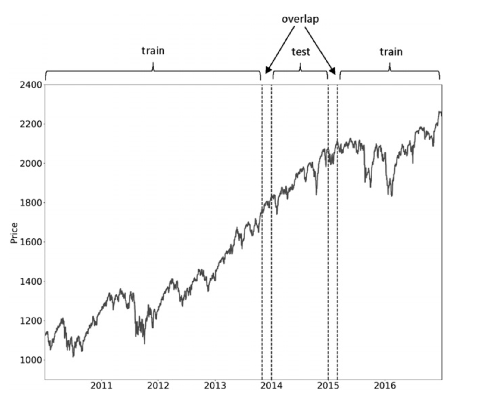
- Purging: This process removes training samples that contain information overlapping with the test set. By eliminating this overlap, purging ensures that the model evaluates unseen data more reliably.
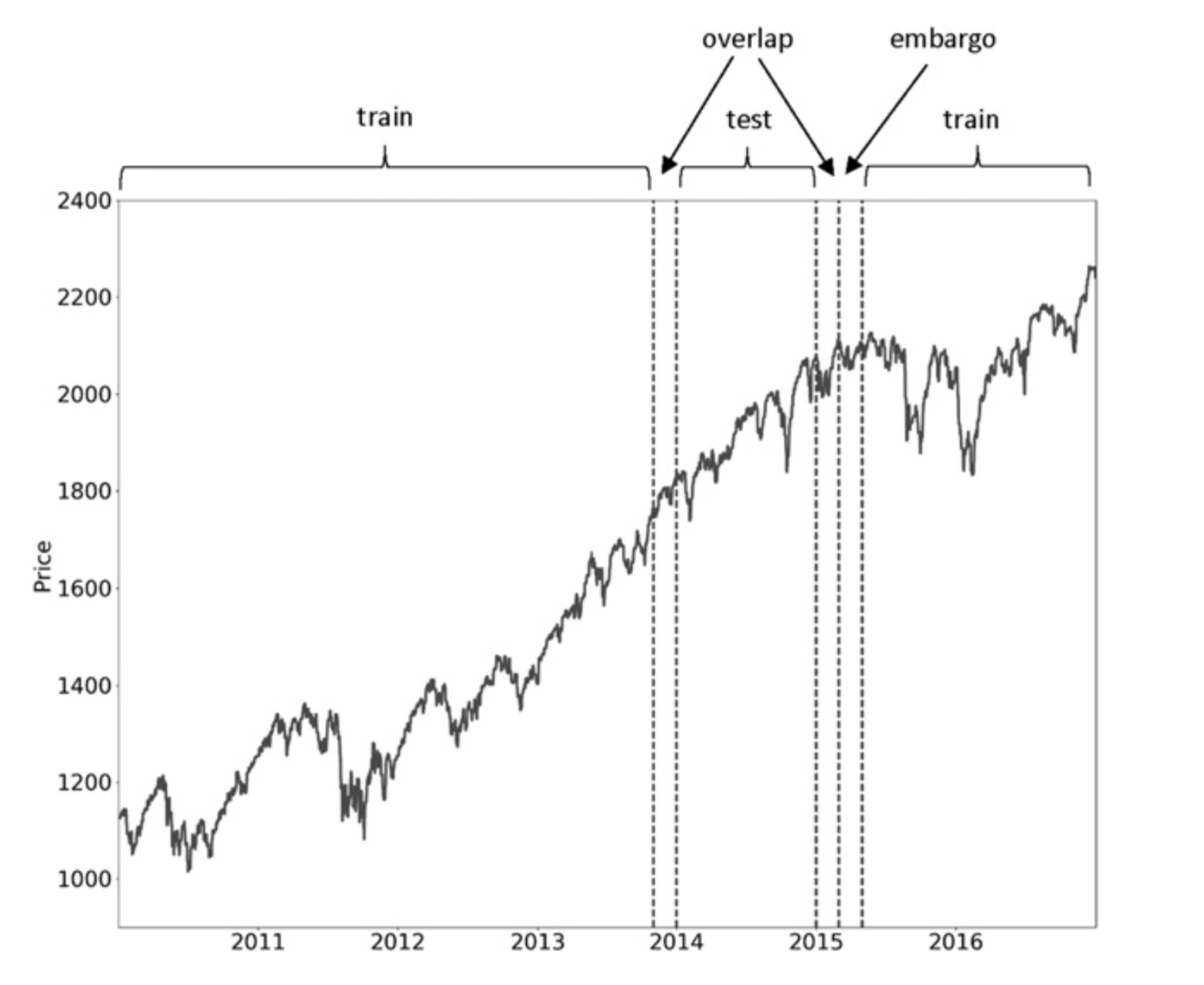
- Embargo: To address potential leakage that purging alone cannot eliminate, embargo excludes a buffer of observations at the end of the test set. This additional safeguard prevents inadvertent use of data that could influence predictions.
Together, these techniques elevate cross-validation to meet the stringent demands of financial machine learning, where even subtle data leakage can lead to flawed conclusions.
Let’s get started.
First, we begin by importing the necessary libraries.
1
2
3
4
5
6
7
8
9
10
11
12
13
14
15
16
17
18
19
20
21
import numpy as np
import pandas as pd
import talib

# Building the Artificial Neural Network
from keras.models import Sequential
from keras.layers import Dense
from keras.layers import Dropout

from itertools import combinations
import itertools as itt
import pyfolio as pf
from tqdm.notebook import tqdm
from hurst import compute_Hc

from sklearn.preprocessing import StandardScaler

import random

import matplotlib.pyplot as plt
from matplotlib.pyplot import cm
Set the random seed to a fixed number.
1
random.seed(42)
Utility Functions for Combinatorial Cross-Validation (CCV)
Purging
This function is adapted from Snippet 7.1 in the Advances in Financial Machine Learning (AFML) book. The purging process eliminates samples from the training set that contain information overlapping with the test set, ensuring a cleaner separation between training and evaluation data.
The function returns a refined training set by removing instances where:
- Training data starts within the test set.
- Training data ends within the test set.
- Training data fully encompasses the test set.
This ensures a strict separation between training and testing data, minimizing information leakage.
1
2
3
4
5
6
7
8
9
def purge(t1, test_times):
    # Whatever is not in the train set should be in the test set
    train = t1.copy(deep=True)
    for test_start, test_end in test_times.items():
        df_0 = train[(test_start <= train.index) & (train.index <= test_end)].index # train starts within test
        df_1 = train[(test_start <= train) & (train <= test_end)].index # train ends within test
        df_2 = train[(train.index <= test_start) & (test_end <= train)].index # train envelopes test
        train = train.drop(df_0.union(df_1).union(df_2))
    return train
Embargo
This function is adapted from Snippet 7.2 in the Advances in Financial Machine Learning (AFML) book.
1
2
3
4
5
6
7
8
def embargo_(times, pct_embargo):
    step = int(times.shape[0] * pct_embargo)
    if step == 0:
        ans = pd.Series(times, index=test_times)
    else:
        ans = pd.Series(times[step:].values, index=times[:-step].index)
        ans = pd.concat([ans, pd.Series(times.iloc[-1], index=times[-step:].index)])
    return ans
Here’s a breakdown of what the above code snippet does:
ans = pd.Series(times[step:].values, index=times[:-step].index)
- It creates a new
pandasSeriesans. - It takes the values from the
timesseries starting from the indexsteponward (times[step:]). - The index for this new Series is set to the index of the original
timesseries, but without the laststepentries (times[:-step].index).
ans = pd.concat([ans, pd.Series(times.iloc[-1], index=times[-step:].index)])
- This appends to the
ansSeries a newpandasSeries created from the last value oftimes(times.iloc[-1]). - The index for this new Series is the last
stepindices of the originaltimesseries (times[-step:].index). - The
pd.concat()function combines both the existingansSeries and the newly created Series, adding the last value fromtimesto the end ofans.
Essentially, it creates a “shifted” version of the series where the data from the original series is moved by step positions, and the last value is retained in the correct place.
Let’s create an example with a pandas Series of 20 entries and demonstrate what the code does with a step value of 5.
Example:
1
2
3
4
5
6
7
8
9
10
11
12
13
14
import pandas as pd

# Create a pandas Series with 20 entries
times = pd.Series(range(1, 21))

# Set step value
step = 5

# Apply the code logic
ans = pd.Series(times[step:].values, index=times[:-step].index)
ans = pd.concat([ans, pd.Series(times.iloc[-1], index=times[-step:].index)])

# Output the result
print(ans)
Explanation:
- The initial series
timeshas 20 values, from 1 to 20. - The code shifts the values by
step(5), so the first 5 values are removed from the start and the last value (times.iloc[-1]) is added at the end.
Expected Output:
1
2
3
4
5
6
7
8
9
10
11
12
13
14
15
16
17
18
19
20
21
0     6
1     7
2     8
3     9
4    10
5    11
6    12
7    13
8    14
9    15
10   16
11   17
12   18
13   19
14   20
15   20
16   20
17   20
18   20
19   20
dtype: int64
Step-by-step breakdown:
- The first line (
times[step:]) starts at index 5 (skipping the first 5 elements), creating a Series from 6 to 20. - The second line (
times[:-step].index) provides the indices from 0 to 14 (effectively dropping the last 5 values). - The last line (
pd.concat([ans, pd.Series(times.iloc[-1], index=times[-step:].index)])) appends the last value (20) at the end, keeping it aligned with the last 5 indices of the original series.
This results in a series where the first 5 entries are shifted out, and the value 20 is appended correctly, matching the last 5 positions of the original series.
The actual embargo function wraps the embargo_ function and applies the embargo to the provided test set (test_times) and time series (t1). It modifies the test set by removing a specified number of observations from its end, determined by the percentage parameter. This ensures additional protection against data leakage, further isolating the test set from any potential influence of future observations.
In the code snippet below, t1 holds both the trade time and the event time.
1
2
3
4
5
def embargo(test_times, t1, pct_embargo=0.01):
    t1_embargo = embargo_(t1, pct_embargo) # Embargoed t1
    # Ensure the output contains only the relevant times that correspond to the indices of test_times.
    test_times_embargoed = t1_embargo.loc[test_times.index]
    return test_times_embargoed
The function returns the embargoed version of test_times, which now excludes some observations from the end, according to the embargo logic.
For example if test_times originally was:
1
2
3
4
test_times:
4    4
5    5
dtype: int64
then after a 25% embargo (i.e. step 5) test_times_embargoed will be:
1
2
3
4
test_times_embargoed:
4    10
5    11
dtype: int64
Combinatorial Cross Validation
One significant limitation of the standard cross-validation (CV) approach in finance is that it evaluates only a single path, which may not fully capture the variability of market dynamics. In the absence of a market simulator, an effective alternative is to leverage combinatorial techniques to generate multiple backtest paths, providing a more robust evaluation framework.
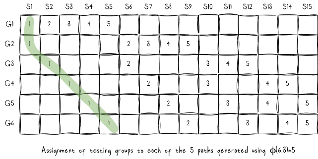
We can also generate multiple fully sampled backtest paths using only the test groups. For instance, a (6,2) split results in five distinct backtest paths.
The figure above illustrates the assignment of each test group to a specific backtest path. For example:
- Path 1 (green) combines forecasts from test groups: (G1, S1), (G2, S1), (G3, S2), (G4, S3), (G5, S4), and (G6, S5).
- Path 2 combines forecasts from test groups: (G1, S2), (G2, S6), (G3, S6), (G4, S7), (G5, S8), and (G6, S9).
This process continues to create additional paths, ensuring diverse and fully sampled backtesting scenarios.
For this section of the blog, I will demonstrate how to construct 5 backtest paths from a single historical path using the combinatorial purged cross-validation (CPCV) framework. This technique is particularly useful for generating diverse backtesting scenarios while minimizing data leakage, as illustrated in the diagram above.
To make the process clear and actionable, I’ll provide a concrete example in Python, walking through the steps required to implement CPCV effectively. Let’s dive into the code!
1
2
3
4
5
6
7
8
9
10
11
12
13
14
15
16
17
18
19
20
21
22
23
24
25
26
27
28
29
30
31
32
33
34
35
36
37
38
39
40
41
42
43
44
45
46
47
48
49
50
51
52
53
54
55
56
57
58
def cpcv_generator(t_span, num_groups, k):
    # Split data into N groups, with N << t_span (i.e. N is significantly less than t_span)
    # This will assign each index position to a group position
    group_num = np.arange(t_span) // (t_span // num_groups)
    group_num[group_num == num_groups] = num_groups-1

    # Generate the combinations
    test_groups = np.array(list(itt.combinations(np.arange(num_groups), k))).reshape(-1, k) # 15×2 matrix: [0,1],[0,2]...[0,5]...[3 5],[4 5]]
    C_nk = len(test_groups)
    n_paths = C_nk * k // num_groups

    print('Number of simulations:', C_nk) # e.g. 15
    print('Number of paths:', n_paths) # e.g. 5

    # is_test is a T x C(n, k) array where each column is a logical array indicating which observation is in the test set
    is_test_group = np.full((num_groups, C_nk), fill_value=False) # 6×15 matrix
    is_test = np.full((t_span, C_nk), fill_value=False) # 100×15 matrix or 7566×15 matrix depending on T

    # Assign test folds for each of the C(n, k) simulations
    for sim_idx, pair in enumerate(test_groups):
        i, j = pair # [0,1], [0,2],... [0,5], [1,2],..., [4,5]
        is_test_group[[i, j], sim_idx] = True # is_test_group is 6×15 matrix.
                                              # Since test_groups is [0,1], [0,2], [0,3], [0,4],... [0,5], [1,2],..., [4,5], simulation with idx 3 will consists of ticks in group 0 and 4 (i.e. the [0,4] pair)
        # Assigning the test folds
        mask = (group_num == i) | (group_num == j) # group_num = [0, 0, ..., 1, 1, ..., 2, 2, ..., 3, 3, ..., 4, 4, ...] of length 100 or 7566 (number of ticks)
                                                   # for [i,j]=[0,4] mask becomes [True, True, ..., False, False, ..., False, False, ..., False, False, ..., True, True, ...]
        is_test[mask, sim_idx] = True # Mark the rows that belong to group i,j so that they belong to sim_idx and are for testing and backtesting.
                                      # For example, since groups [0,4] belong to simulation 3, we set simulation 3 to True for all the rows that belong to group 0 or 4 to indicate that they should be used
                                      # for testing in simulation 3

    # For each path, connect the folds from different simulations to form a test path.
    # The fold coordinates are: the fold number, and the simulation index e.g. simulation 0, fold 0 etc
    path_folds = np.full((num_groups, n_paths), fill_value=np.nan)
    for p in range(n_paths):
        for group in range(num_groups):
            # The argmax() function explained: assuming is_test_group[group, :]=[F, F, F, T, F, F, F, T, F, F, T, F, T, F, T] then argmax() returns sim_idx=3
            sim_idx = is_test_group[group, :].argmax().astype(int)
            path_folds[group, p] = sim_idx  # Considering the above example where sim_idx=3 is associated with groups [0,4]:
                                            #     path_folds[0,0], path_folds[0,1],..., path_folds[0,4] will be set to sim_idx=3
                                            # Same for group 4:
                                            #     path_folds[4,0], path_folds[4,1],..., path_folds[4,4] will be set to sim_idx=3

            # Mark it as False so on the next iteration we get the next sim_idx when doing a "...argmax().astype(int)" (e.g. sim_idx=7)
            is_test_group[group, sim_idx] = False


    # Finally, for each path we indicate which simulation we're building the path from and the time indices
    paths = np.full((t_span, n_paths), fill_value= np.nan) # 100×15 matrix or 7566×5 matrix
    for p in range(n_paths):
        for g in range(num_groups):
            mask = (group_num == g) # Get all the ticks that belong to group g
            paths[mask, p] = int(path_folds[g, p])

    # Once done the matrices will look like so:
    # is_test[99] = [F, F, F, F, True, F, F, F, True, F, F, True, F, True, True]
    # paths[99] = [4, 8, 11, 13, 14]
    # path_folds[5] = [4, 8, 11, 13, 14]
    return (is_test, paths, path_folds)
To use the function described above, simply execute the following:
1
2
3
4
5
6
7
num_ticks = 100
num_paths = 5
num_groups_test = 2
num_groups = num_paths + 1

# path_folds will be discared we are only interested in it because we want to test it against our hardcoder matrtix [[ 0.,  1.,  2.,  3.,  4.],...]
is_test, paths, path_folds = cpcv_generator(num_ticks, num_groups, num_groups_test)
This is quite a bit of code, so rather than getting into the specifics of Pandas and NumPy, I’ll focus on giving you a clear understanding of the core concept. To help you follow along, I’ve included detailed comments with each line of code to explain what’s happening step by step. Make sure to read through the comments for additional clarity.
is_test
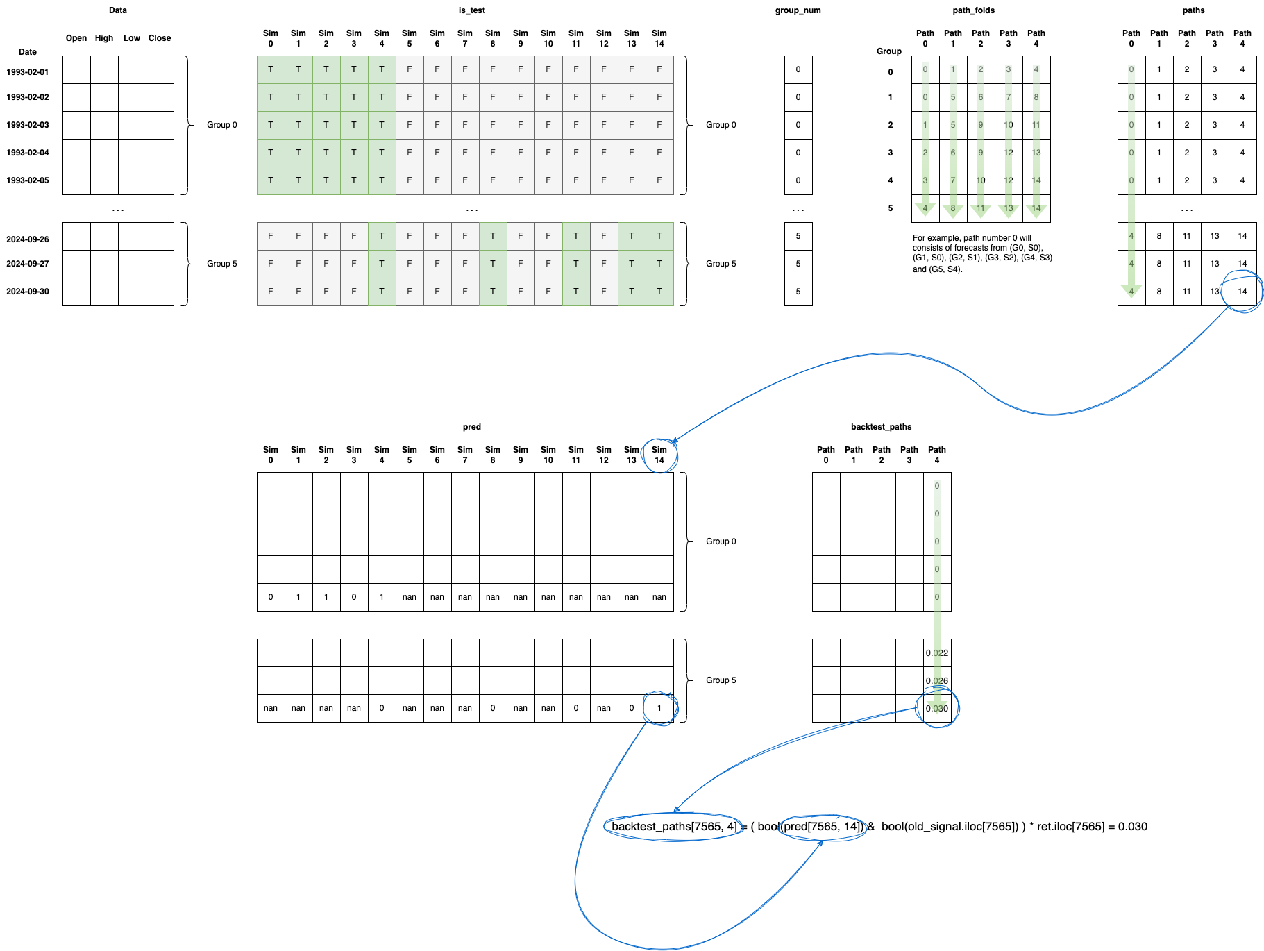
Has tick-number of rows, with each row pointing to a number-of-sims long array, marking the simulation to be used as True. For example assuming:
1
2
3
4
5
...
is_test[50] = [F, F, T, F, F, F, T, F, F, F, F, F, T, T, F]
...
is_test[99] = [F, F, F, F, T, F, F, F, T, F, F, T, F, T, T]
...
above, we read columnwise for each of the 15 simulations. In simulation index 2, tick number 50 will be considered for testing/backtesting, while tick 99 will not. On the other hand in simulation 4 tick 99 will be used for test while tick 50 will not.
paths
Has tick-number of rows and 5 columns. Each column represents one path (again, we read column wise) . A path consist of simulation indices. Example: paths[99] = [4, 8, 11, 13, 14]. In this example, tick 99 is part of 5 paths. In the first path we will consider the prediction of simulation 4. In the second path we will consider the prediction of simulation 8, and so on. It will be used for the backtesting after we have trained (using training set) and predicted using the test set. In other words, if our prediction (pred) matches the real signal (old_signal) then backtest_paths[tick, p] will hold the return that we would gain. This logic is depicted below:
1
2
3
for p in range(paths.shape[1]):
    for t, sim in enumerate(paths[:, p]): # index, value
        backtest_paths[t, p] = ( bool(pred[t, int(sim)]) &  bool(old_signal.iloc[t]) ) * ret.iloc[t]
pred has tick-number of rows and number-of-sims columns filled as follows:
1
2
3
4
for sim in range(num_sim):
    test_idx = is_test[:, sim]
    ...
    pred[test_idx, sim] = classifier.predict(X_test)
Finally, I’ve included an illustration to help you visualize the process. The diagram is organized to be read from left to right, top to bottom and provides a clear depiction of each step. It shows how the data is structured and manipulated within the NumPy arrays, giving you a comprehensive view of how everything is laid out and interconnected.
Read the Data
1
2
3
4
5
# Read the data from CSV file
data = pd.read_csv('aapl_prices.csv', parse_dates=True, sep=',', index_col=[0])
data.index = pd.to_datetime(data.index)
data = data.dropna()
data.head()
| Close | Volume | Open | High | Low | |
|---|---|---|---|---|---|
| Date | |||||
| 2020-02-28 | 273.36 | 106721200 | 257.26 | 278.41 | 256.37 |
| 2020-02-27 | 273.52 | 80151380 | 281.10 | 286.00 | 272.96 |
| 2020-02-26 | 292.65 | 49678430 | 286.53 | 297.88 | 286.50 |
| 2020-02-25 | 288.08 | 57668360 | 300.95 | 302.53 | 286.13 |
| 2020-02-24 | 298.18 | 55548830 | 297.26 | 304.18 | 289.23 |
1
2
3
spy_data = pd.read_csv('spy_prices.csv', parse_dates=True, sep=',', index_col=[0])
spy_data = spy_data.loc[data.index]
spy_data.head()
| Open | High | Low | Close | Volume | Day | Weekday | Week | Month | Year | |
|---|---|---|---|---|---|---|---|---|---|---|
| Date | ||||||||||
| 2020-02-28 | 268.561652 | 277.110603 | 265.622075 | 275.594299 | 384975800 | 28 | 4 | 9 | 2 | 2020 |
| 2020-02-27 | 284.152539 | 289.827037 | 276.757111 | 276.757111 | 284353500 | 27 | 3 | 9 | 2 | 2020 |
| 2020-02-26 | 292.264289 | 295.920144 | 289.027056 | 289.771240 | 194773800 | 26 | 2 | 9 | 2 | 2020 |
| 2020-02-25 | 301.343506 | 301.966754 | 289.948007 | 290.841034 | 218913200 | 25 | 1 | 9 | 2 | 2020 |
| 2020-02-24 | 300.599312 | 310.292447 | 298.831824 | 299.929535 | 161088400 | 24 | 0 | 9 | 2 | 2020 |
Preparing the Dataset
1
2
3
4
5
6
7
8
9
10
11
12
13
14
15
16
17
18
19
data['H-L'] = data['High'] - data['Low']
data['O-C'] = data['Close'] - data['Open']
data['3day MA'] = data['Close'].shift(1).rolling(window = 3).mean()
data['10day MA'] = data['Close'].shift(1).rolling(window = 10).mean()
data['30day MA'] = data['Close'].shift(1).rolling(window = 30).mean()
data['21day MA'] = data['Close'].shift(1).rolling(21).mean()
data['263day MA'] = data['Close'].shift(1).rolling(262).mean()
data['Std_dev']= data['Close'].rolling(5).std()
data['RSI'] = talib.RSI(data['Close'].values, timeperiod = 9)
data['Williams %R'] = talib.WILLR(data['High'].values, data['Low'].values, data['Close'].values, 7)
data['zscore'] = (data.Close - data.Close.rolling(126).mean())/data.Close.rolling(126).std()
data['hurst'] = data['Close'].rolling(window=126).apply(lambda x: compute_Hc(x)[0])

data['High_std'] = (data['High']-data['High'].mean())/data['High'].std()
spy_data['High_std'] = (spy_data['High']-spy_data['High'].mean())/spy_data['High'].std()
data['aapl-spy'] = data['High_std'] - spy_data['High_std']

# 21 days holding period
data['returns'] = data.Close.shift(-21).ffill().pct_change(21)
Defining Input Features from a Dataset
1
2
3
4
5
6
7
data['Price_Rise'] = np.where(data['Close'].shift(-21) > data['Close'], 1, 0)
data = data.dropna()

feats = ['zscore', 'aapl-spy']
#feats = ['zscore', 'Std_dev', '21day MA', '263day MA']
X = data[feats]
y = data['Price_Rise']
Building the Neural Network Model
1
2
3
4
5
6
7
8
9
10
11
12
13
14
15
16
17
18
19
20
21
22
23
24
25
26
27
28
29
30
31
32
33
34
35
36
37
38
39
40
41
42
43
44
45
46
47
48
49
50
51
52
53
54
55
56
57
58
59
60
61
62
63
64
65
# Prediction and evaluation times using business days, but the index is not holidays aware -- it can be fixed
t1_ = data.index

# We are holding our position for 21 days
t1 = pd.Series(t1_[21:], index=t1_[:-21]) # t1 is both the trade time and the event time

# Realign data
data = data.loc[t1.index]

data = data.dropna()

# Realign t1
t1 = t1.loc[data.index]

num_paths = 5
num_groups_test = 2
num_groups = num_paths + 1
num_ticks = len(data)
is_test, paths, _ = cpcv_generator(num_ticks, num_groups, num_groups_test)
pred = np.full(is_test.shape, np.nan)

num_sim = is_test.shape[1] # num of simulations needed to generate all backtest paths
for sim in tqdm(range(num_sim)):
    # Get train set|
    test_idx = is_test[:, sim]

    # Convert numerical indices into time stamps
    test_times = t1.loc[test_idx]

    # Embargo
    test_times_embargoed = embargo(test_times, t1, pct_embargo=0.01)

    # Purge
    train_times = purge(t1, test_times_embargoed)

    # Split training / test sets
    X_test = X.loc[test_times.index, :]
    y_test = y.loc[X_test.index]

    X_train = X.loc[train_times.index, :]
    y_train = y.loc[X_train.index]

    sc = StandardScaler()

    X_train = sc.fit_transform(X_train)
    X_test = sc.transform(X_test)

    # Reconstructing the backtest paths
    print(f'training classifier for simulation %s' % sim)
    np.random.seed(42)

    classifier = Sequential()
    classifier.add(Dense(units = 128, kernel_initializer = 'uniform', activation = 'relu', input_dim = X.shape[1]))
    classifier.add(Dense(units = 128, kernel_initializer = 'uniform', activation = 'relu')) # second layer
    classifier.add(Dense(units = 1, kernel_initializer = 'uniform', activation = 'sigmoid')) # output layer
    classifier.compile(optimizer = 'adam', loss = 'mean_squared_error', metrics = ['accuracy']) #  ‘adam’ is stochastic gradient descent.
    classifier.fit(X_train, y_train, batch_size = 10, epochs = 100, verbose=0)

    pred_ = classifier.predict(X_test)
    pred_ = np.concatenate(pred_, axis=0)

    pred_ = (pred_ > 0.5)

    # Fill the backtesting prediction matrix
    pred[test_idx, sim] = pred_
1
2
3
4
5
6
7
8
9
10
11
12
Number of simulations: 15
Number of paths: 5

24/24 ━━━━━━━━━━━━━━━━━━━━ 0s 1ms/step
training classifier for simulation 1

24/24 ━━━━━━━━━━━━━━━━━━━━ 0s 1ms/step
training classifier for simulation 2

...

24/24 ━━━━━━━━━━━━━━━━━━━━ 0s 1ms/step
Calculating Strategy Returns for Each Backtest Path
1
2
3
4
5
backtest_paths = np.full((paths.shape[0], paths.shape[1]), np.nan)

for p in range(paths.shape[1]):
    for t, sim in enumerate(paths[:, p]): # index, value
        backtest_paths[t, p] =  np.where(pred[t, int(sim)] == True, data.iloc[t]['returns'], -data.iloc[t]['returns'])
Computing Performance Metrics for Multiple Backtest Paths
1
2
3
4
5
6
7
8
9
perf_func = pf.timeseries.perf_stats

perf_list = []
for s in range(paths.shape[1]):
    perf_table = perf_func(backtest_paths[:, s])
    perf_list.append(perf_table)

perf_paths = pd.concat(perf_list, axis=1)
perf_paths
| 0 | 1 | 2 | 3 | 4 | |
|---|---|---|---|---|---|
| Annual return | 4.400125e+00 | 0.808613 | -0.372753 | -0.460721 | 0.258365 |
| Cumulative returns | 3.131295e+06 | 190.606415 | -0.984024 | -0.995817 | 6.676995 |
| Annual volatility | 1.184233e+00 | 1.191016 | 1.193744 | 1.193836 | 1.192373 |
| Sharpe ratio | 2.027053e+00 | 1.096188 | 0.214445 | 0.085223 | 0.791091 |
| Calmar ratio | 4.402061e+00 | 0.809866 | -0.372753 | -0.460721 | 0.258366 |
| Stability | 8.500589e-01 | 0.497443 | 0.381901 | 0.450990 | 0.049584 |
| Max drawdown | -9.995602e-01 | -0.998453 | -1.000000 | -1.000000 | -1.000000 |
| Omega ratio | 1.383296e+00 | 1.191707 | 1.034900 | 1.013726 | 1.134919 |
| Sortino ratio | 3.060563e+00 | 1.636466 | 0.302078 | 0.121184 | 1.173034 |
| Skew | -2.446451e-01 | -0.041749 | -0.133953 | -0.024305 | 0.003253 |
| Kurtosis | 3.435320e-01 | 0.224670 | 0.218389 | 0.211606 | 0.211486 |
| Tail ratio | 1.151994e+00 | 1.143523 | 0.991613 | 0.993902 | 1.170246 |
| Daily value at risk | -1.396402e-01 | -0.144839 | -0.149348 | -0.149972 | -0.146448 |
1
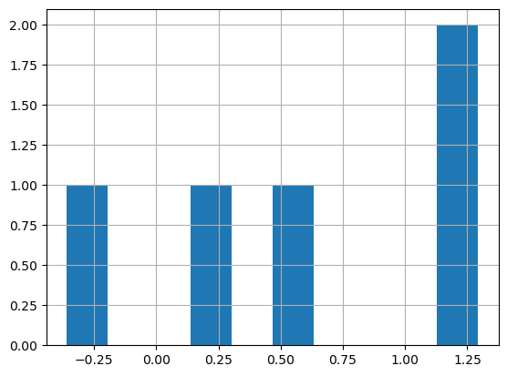
perf_paths.loc['Sharpe ratio', :].mean()
1
0.5726126186562848
1
perf_paths.loc['Sharpe ratio', :].std()
1
0.7050751454073455
1
perf_paths.loc['Sharpe ratio', :].hist()
1
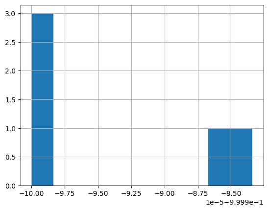
perf_paths.loc['Max drawdown', :].mean()
1
-0.9999935745391175
1
perf_paths.loc['Max drawdown', :].std()
1
8.221205201086146e-06
1
perf_paths.loc['Max drawdown', :].hist()
Calculating and Plotting Cumulative Market and Strategy Returns for Multiple Paths
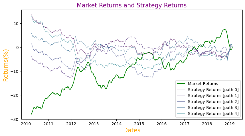
We will now compute the cumulative returns for both the market and the strategy, utilizing the cumsum() function. These cumulative values will be used in the final step to plot the graph of market and strategy returns.
1
2
3
4
5
6
7
8
9
10
11
12
13
14
15
16
17
18
19
20
21
22
23
24
25
26
data['cumulative_market_returns'] = np.cumsum(data['returns'])

strategy_returns = np.full((paths.shape[0], paths.shape[1]), np.nan)
for p in range(paths.shape[1]):
    for t, sim in enumerate(paths[:, p]): # index, value
        strategy_returns[t, p] =  np.where(pred[t, int(sim)] == True, data.iloc[t]['returns'], -data.iloc[t]['returns'])

for p in range(paths.shape[1]):
    data[f'cumulative_strategy_returns_{p}'] = np.cumsum(strategy_returns[:, p])

plt.figure(figsize=(10,5))
plt.plot(data['cumulative_market_returns'], color='g', label='Market Returns')

color = iter(plt.colormaps.get_cmap('viridis').resampled(10).colors)
for p in range(paths.shape[1]):
    c = next(color)
    plt.plot(data[f'cumulative_strategy_returns_{p}'], color=c, label=f'Strategy Returns [path {p}]',linewidth=0.5)

plt.title('Market Returns and Strategy Returns', color='purple', size=15)

# Setting axes labels for close prices plot
plt.xlabel('Dates', {'color': 'orange', 'fontsize':15})
plt.ylabel('Returns(%)', {'color': 'orange', 'fontsize':15})

plt.legend()
plt.show()

