Cointegration Analysis of GLD and GDX for Pair Trading Strategy

Cointegration Analysis of GLD and GDX for Pair Trading Strategy

In this research I am going to test whether the price series of two securities GLD (Gold Price) and GDX (Gold Miners Equity ETF) are cointegrated. This is crucial if we want to develop a pair trading strategy around those two securities. I want to test if the spread between the two series is stationary around its mean. For my pair trading strategy I want the two securities to be cointegrated. For my research I am using Python.

Import The Necessary Python Modules

%matplotlib inline

import pandas as pd
import numpy as np
import matplotlib.pyplot as plt
import math
from sklearn import linear_model
from statsmodels.tsa.stattools import coint
import statsmodels.api as sm
from datetime import timedelta, date

Read GLD and GDX Data

# Read the price series from CSV

def read_prices(): # Read GLD
gld_df = pd.read_csv('GLD.csv', index_col='Date')
gld_df.index = pd.to_datetime(gld_df.index, format = '%Y-%m-%d')

    # Read GDX
    gdx_df = pd.read_csv('GDX.csv', index_col='Date')
    gdx_df.index = pd.to_datetime(gdx_df.index, format = '%m/%d/%Y')

    return (gld_df, gdx_df)

gld_df, gdx_df = read_prices()

Find the intersection of the two

# Select only the prices in the given date range and

# intersect the two prece series

def intersect(gld_df, gdx_df, start_date='2017-01-01', end_date='2018-01-01'):
gld_df = gld_df[start_date:end_date]
gdx_df = gdx_df[start_date:end_date]

    GDX = gdx_df['Close']
    GLD = gld_df['Close']

    GDX = GDX.dropna()
    GLD = GLD.dropna()

    # Find the intersection of the two data sets
    gdx_gld_index_intersection = GLD.index.intersection(GDX.index)

    GDX = GDX.loc[gdx_gld_index_intersection]
    GLD = GLD.loc[gdx_gld_index_intersection]

    return (GDX, GLD)

Next, for the sake of this example, I am going to do an exhaustive search to find a time period when the GLD and GDX price series were cointegrated. Don’t worry about the cointegration test for now. More on that later.

# Brute force search for date ranges where the price series are cointegrated

def get_cointegration_period(start_date=date(2013, 1, 1), end_date=date(2018, 1, 1)):
def daterange(start_date, end_date):
for n in range(int((end_date - start_date).days)):
yield start_date + timedelta(n)

    dates = []
    for single_date in daterange(start_date, end_date):
        dates.append(single_date)

    for i, start_date in enumerate(dates):
        for end_date in dates[i+1:]:
            delta = int((end_date - start_date).days)
            if delta >= 200:
                GDX, GLD = intersect(gld_df, gdx_df, start_date, end_date)

                # Compute the p-value of the cointegration test
                # It will inform us as to whether the spread between the 2 timeseries is stationary
                # around its mean
                alpha = 0.05
                score, pvalue, _ = coint(GDX, GLD)
                if pvalue <= alpha:
                    return (start_date, end_date)

start_date, end_date = get_cointegration_period()
print("The two series are cointegrated during the period %s - %s" % (start_date, end_date))
GDX, GLD = intersect(gld_df, gdx_df, start_date, end_date)

The two series are cointegrated during the period 2013-01-01 - 2017-10-02

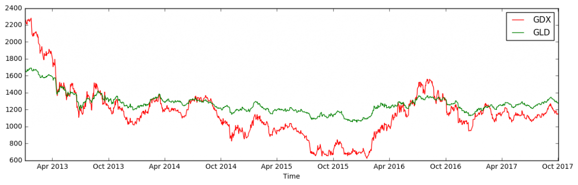
Next, I am going to perform a LinearRegression in order to find a β such that:

\[GLD = β \times GDX\]

I do this so that I can bring the two values on a notionally common scale.

# Do a Linear Regression to find beta such that

# GLD = beta * GDX + e

train_len = len(GLD)//2
results = sm.OLS(GLD[:-train_len], GDX[:-train_len]).fit()
predictions = results.predict(GDX[-train_len:])
beta = results.params[0]
#results.summary()

plt.figure(figsize=(14,4))
plt.plot(GDX \* beta, 'r')
plt.plot(GLD, 'g')
plt.xlabel('Time')
plt.legend(['GDX', 'GLD'])
plt.show()

Testing For Cointegration Between GLD and GDX

Statistical stationarity: A stationary time series is one whose statistical properties such as mean, variance, autocorrelation, etc. are all constant over time. A stationarized series is relatively easy to predict: you simply predict that its statistical properties will be the same in the future as they have been in the past!

The two series are cointegrated if the difference between the two (spread) is mean reverting. Any series that hovers around some mean is mean reverting. That is, it will always revert back to its mean. Here the difference between GLD and GDX hovers around some mean.

plt.figure(figsize=(14,4))
(GLD - GDX).plot() # Plot the spread

plt.axhline((GLD - GDX).mean(), color='red', linestyle='--') # Add the mean
plt.xlabel('Time')
plt.title("Spread Between GLD and GDX")
plt.legend(['Price Spread', 'Mean'])

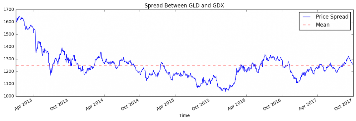
Just by eyeballing the above plot, we can already see that GLD and GDX are cointegrated (for the given time interval). But it is always good to do some hypothesis testing as well, in order to prove that assumption.

Hypothesis Testing for Cointegration

How do we test for cointegration? There is a convenient cointegration test, coint(...) that lives in statsmodels.tsa.stattools.

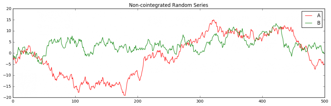
Before I test for cointegration using coint(...), I need to know what the null hypothesis H0 is, that coint(...) is testing. For that, I am going to test A and B, two series that are obviously not related. Since A and B are not related, I would expect that coint(A, B) would indicate so.

A, B = np.random.randn(2, 500).cumsum(1)

plt.figure(figsize=(14,4))
plt.title("Non-cointegrated Random Series")
plt.plot(A, 'r')
plt.plot(B, 'g')
plt.legend(['A', 'B'])
plt.show()

Let us see if the spread between A and B is mean reverting:

# Plot the spread

plt.figure(figsize=(14,4))
plt.plot((A - B))
plt.axhline((A - B).mean(), color='red', linestyle='--') # Add the mean
plt.title("A-B Spread and Spread Mean")
plt.legend(['A - B Spread', 'Mean'])

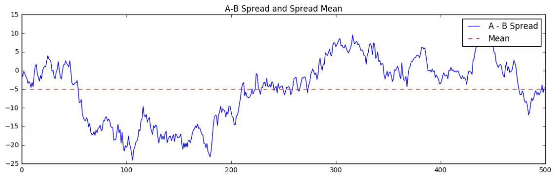
We can see that the spread is clearly not mean reverting. Now, let’s have a look at the p-value resulting from coint(A,B)

_, pvalue, _ = coint(A, B)
print("p-value: %s" % pvalue)

p-value: 0.749539065377

We can see that the test spit out a p-value of around 0.9. Recall the definition of p-value:

The p-value, or calculated probability, is the probability of finding the observed, or more extreme, results when the null hypothesis (H0) of a study question is true.

In other words, assuming A and B are not cointegrated (that is, assume H0 is true) how likely (p-value) is it to get the observed data? If the p-value is small (typically ≤ 0.05), then it indicates that it is very unlikely to get such extremes and so we reject the null hypothesis.

Since, in our test case we actually know that A and B are not cointegrated and the resulting p-value is 0.9, we can be sure that coint(A,B) tests the following hypotheses:

• H0: A and B are not cointegrated.
• Ha: A and B are cointegrated.

We set our alpha level to 0.05. That is, assuming that the null hypothesis is true, this means we may reject the null only if the observed data are so unusual that they would have occurred by chance at most 5% of the time.

So for the case A and B we wouldn’t reject the null hypotheses, “X and Y are not cointegrated”, since the resulting p-value is >= 0.05.

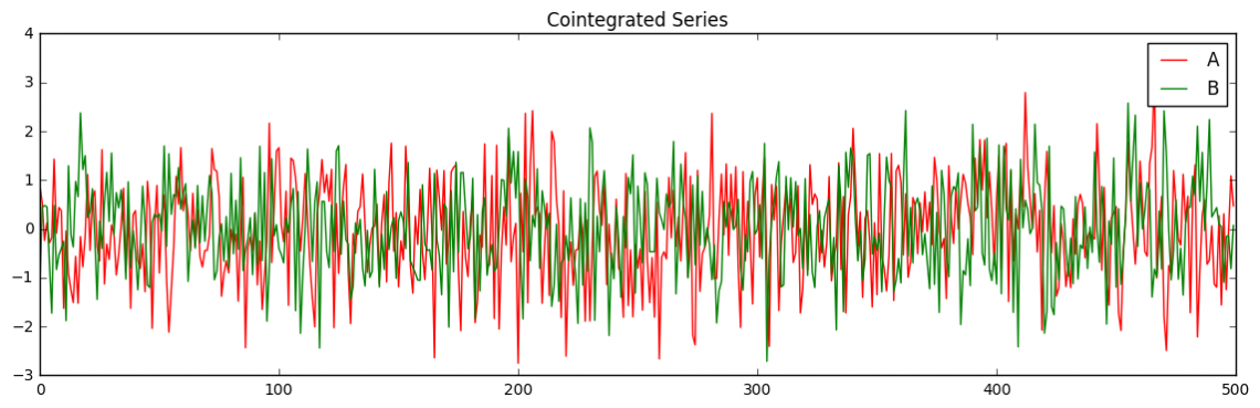
Let us look at another example. This time with cointegrated data:

A, B, Z = np.random.randn(3, 500)
plt.figure(figsize=(14,4))
plt.title("Cointegrated Series")
plt.plot(A, 'r')
plt.plot(B, 'g')
plt.legend(['A', 'B'])
plt.show()

Let us see if the spread between A and B is mean reverting. That is, it hovers around some mean:

# Plot the spread

plt.figure(figsize=(14,4))
plt.plot((A - B))
plt.axhline((A - B).mean(), color='red', linestyle='--') # Add the mean
plt.title("A-B Spread and Spread Mean")
plt.legend(['A - B Spread', 'Mean'])

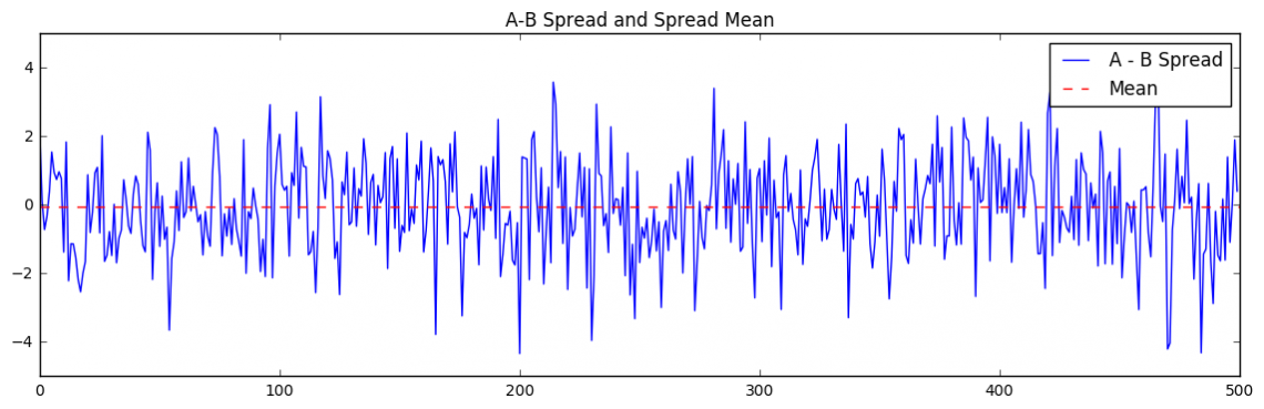
We can see that the spread is indeed mean reverting. Let’s have a look at the p-value resulting from coint(A,B):

_, pvalue, _ = coint(A+Z, B+Z)
print("p-value: %s" % pvalue)

p-value: 0.000853541266594

We can see that when the series are cointegrated, coint(...) spits out a smaller p-value. Again, running it through the test:

“Assuming A and B are not cointegrated (that is, assume H0 is true) how likely (p-value) is it to get the observed data?”

Since the resulting p-value is very small (around 0.0002), it indicates that it is very unlikely that we get the observed data (which we know is cointegrated) if the series are not cointegrated. Which proves our assumption that the null hypotheses tested by coint(...) is indeed: “A and B are not cointegrated”.

Back to our original series GDX and GLD we would reject the null hypotheses “GDX and GLD are not cointegrated” and go for the alternative hypotheses Ha: “GDX and GLD are cointegrated” if the resulting p-value is ≤ 0.05. Again, this is because coint(...) tests for no-cointegration:

# Compute the p-value of the cointegration test

# It will inform us as to whether the spread between the 2 timeseries is stationary

# around its mean

alpha = 0.05
score, pvalue, \_ = coint(GDX, GLD)
if pvalue <= alpha:
print("The two series are cointegrated (p-value: %s)" % pvalue)
else:
print("The two series are not cointegrated (p-value: %s)" % pvalue)

The two series are cointegrated (p-value: 0.0480429692164)

Running the cointegration test we can see that GLD and GDX are cointegrated.

Creating a Pair Trading Strategy

For my next research I am going to develop a pair trading strategy where I am going to:

• Long GLD and short GDX when the spread gets narrow (spread-z-score <= -t)
• Long GDX and short GLD when the spread gets wide (spread-z-score <= t)

with spread = GLD – β * GDX. The reasoning behind this strategy is that we are hoping that eventually the spread will revert to its mean. For example if the spread gets narrow, this can happen due to the following reasons:

• GLD’s price dropped and GDX didn’t change. In that case I make money when GLD reverts back to its mean (i.e. goes back up), because I go long GLD.
• GLD’s price dropped and GDX’s price increased. In that case I make money when GLD reverts back to its mean (i.e. goes back up) and GDX also reverts to its mean (i.e. drops back down), because I go long GLD and short GDX.
• Also, since I make a pairs trade by buying one security and selling another, if both securities go down together or go up together, I neither make nor lose money — I am market neutral.