Implementing a Neural Network from Scratch in Python (Part 2)

Implementing a Neural Network from Scratch in Python (Part 2)

GitHub repository

In this example, we’ll examine sales based on the ‘TV’ marketing budget. Our goal is to train a neural network model to predict ‘Sales’ using ‘TV’ as the predictor variable. You can download the advertising dataset here.

Let’s start by visualizing the relationship between the feature and the response variable with a scatterplot:

From the plot, it’s clear that as the TV budget increases, sales tend to rise as well. Now, let’s train our neural network to see if it can accurately capture this relationship.

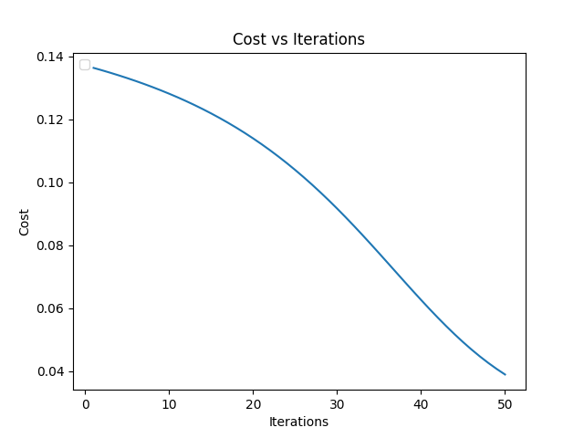
We’ll start by reading in the data and running the training for an initial 50 iterations. We also plot the neural network cost $J$ against the number of iterations.

from neural_network import Neural_Network
import matplotlib.pyplot as plt
import pandas as pd
import numpy as np
from sklearn.model_selection import train_test_split

topology = {
    'input_layer_size': 1,
    'number_of_hidden_layers': 1,
    'hidden_layer_size': 3,
    'output_layer_size': 1
}

def train():
    NUMBER_OF_WEIGHTS = (topology['input_layer_size'] * topology['hidden_layer_size']) + (topology['number_of_hidden_layers']-1) * (topology['hidden_layer_size']**2) + (topology['hidden_layer_size'] * topology['output_layer_size'])
    advertising = pd.read_csv('tvmarketing.csv')
    X = advertising['TV'].to_numpy()
    y = advertising['Sales'].to_numpy()

    X_train, X_test, y_train, y_test = train_test_split(X, y, train_size=0.7 , random_state=0000)

    X_train = np.array([[x] for x in X_train])
    y_train = np.array([[y] for y in y_train])

    X_test = np.array([[x] for x in X_test])
    y_test = np.array([[y] for y in y_test])

    # Rule-of-thumb is that the sample size needs to be at least a factor 10 times the number
    # of weights in the network (Abu-Mostafa, 1995; Baum and Haussler, 1989; Haykin, 2009)
    if X_train.shape[0] >= 10 * NUMBER_OF_WEIGHTS:
        NUMBER_OF_ITERATIONS = 50
        net = Neural_Network(topology=topology, delete_old_db=True)

        X_train_scaled, y_train_scaled = net.transform(X=X_train, y=y_train)

        print("Training neural network using gradient descent...")
        J = []
        for i in range(NUMBER_OF_ITERATIONS):
            net.train_using_gradient_descent(X_train_scaled, y_train_scaled)
            J.append(net.cost_function(X_train_scaled, y_train_scaled))

        # Plot Cost vs Iterations
        plt.plot([i for i in range(1, NUMBER_OF_ITERATIONS+1)], J)
        plt.xlabel('Iterations')
        plt.ylabel('Cost')
        plt.title('Cost vs Iterations')
        plt.legend(loc="upper left")
        plt.show()

        cost = net.cost_function(X_train_scaled, y_train_scaled)
        print(f"Final cost: {cost}")
        return X_test, y_test
    else:
        print(f"Not enough samples. Need at least {10*NUMBER_OF_WEIGHTS}. Exiting.")

if __name__ == "__main__":
    X_test, y_test = train()

I think we can do better than that. Lets try with 200 iterations.

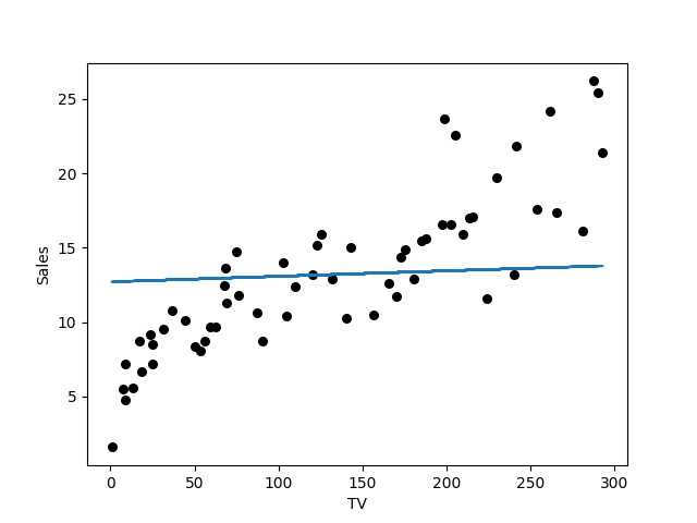
That looks better. Let us try to predict something.

def test(X_test, y_test):
    net = Neural_Network(topology=topology)

    fig = plt.figure()
    ax = fig.add_subplot(111)

    ax.scatter(X_test[:, 0], y_test, c='k', alpha=1, s=30)

    X_test_scaled, y_test_scaled = net.transform(X=X_test, y=y_test)
    yHat = net.forward(X_test_scaled)

    # Unscale
    yHat = np.min(y_test, axis=0) + yHat * (np.max(y_test, axis=0) - np.min(y_test, axis=0))

    ax.plot(X_test[:, 0], yHat)
    ax.set_xlabel('TV')
    ax.set_ylabel('Sales')

    plt.show()

if __name__ == "__main__":
    X_test, y_test = train()
    test(X_test, y_test)

This doesn’t look good. Let us train it again. This time with 1000 iterations.

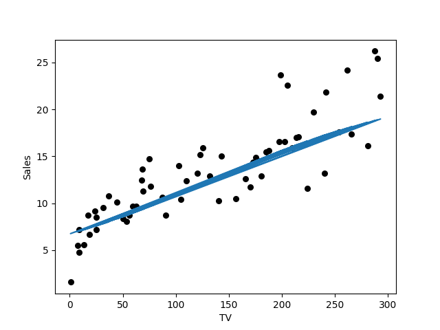
We are not quite there yet. Let’s try this again with 10000 iterations.

We’re definitely seeing improvement now! Our model is accurately capturing the relationship between the TV budget and Sales. In this example, we used a simple structure: one input neuron, one output neuron, and a hidden layer with three neurons. Feel free to experiment with different network topologies to observe how they impact performance.